How to use Sverchok to create raster Voronoi patterns for 3d printing and CNC milling.

The partitioning of a plane with n points into convex polygons such that each polygon contains exactly one generating point and every point in a given polygon is closer to its generating point than to any other.
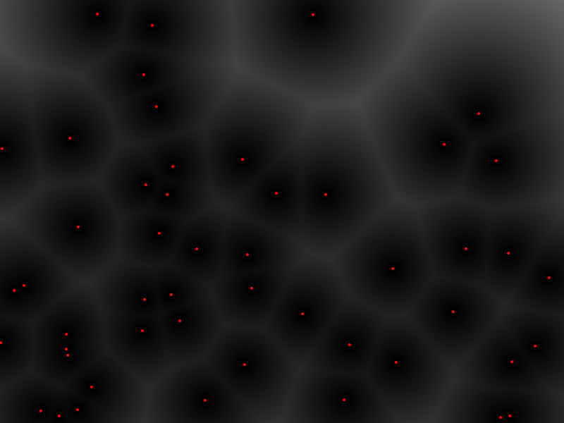
This is the definition of the Voronoi diagram, according to the Wolram Notebook. While getting the vector coordinates of the diagram requires quite complicated algorithms (at least for me), the procedure to display the polygons inside a discrete raster image is fairly intuitive and simple. All we need to do is loop though every pixel and assign to it a color that represents the distance from its closest point within the given input points. In fact, we can do this in few lines of Processing.
void setup() {
  size(800, 600);
  background(255);

  PVector[] points = new PVector[50];

  for (int i=0; i<points.length; i++) {
    points[i] = new PVector(random(width), random(height));
  }

  float max_dist = sqrt(sq(width)+sq(height)) / 2;

  loadPixels();
  for (int y=0; y<height; y++) {
    for (int x=0; x<width; x++) {
      PVector pixel = new PVector(x, y);
      float min_dist = Float.MAX_VALUE;
      for (PVector p : points) {
        float dist = dist(pixel.x, pixel.y, p.x, p.y);
        min_dist = dist < min_dist ? dist : min_dist;
      }
      pixels[width*y+x] = color(map(min_dist, 0, max_dist, 0, 255));
    }
  }
  updatePixels();

  fill(255,0,0);
  for (PVector p : points) {
    ellipse(p.x, p.y, 5, 5);
  }
}
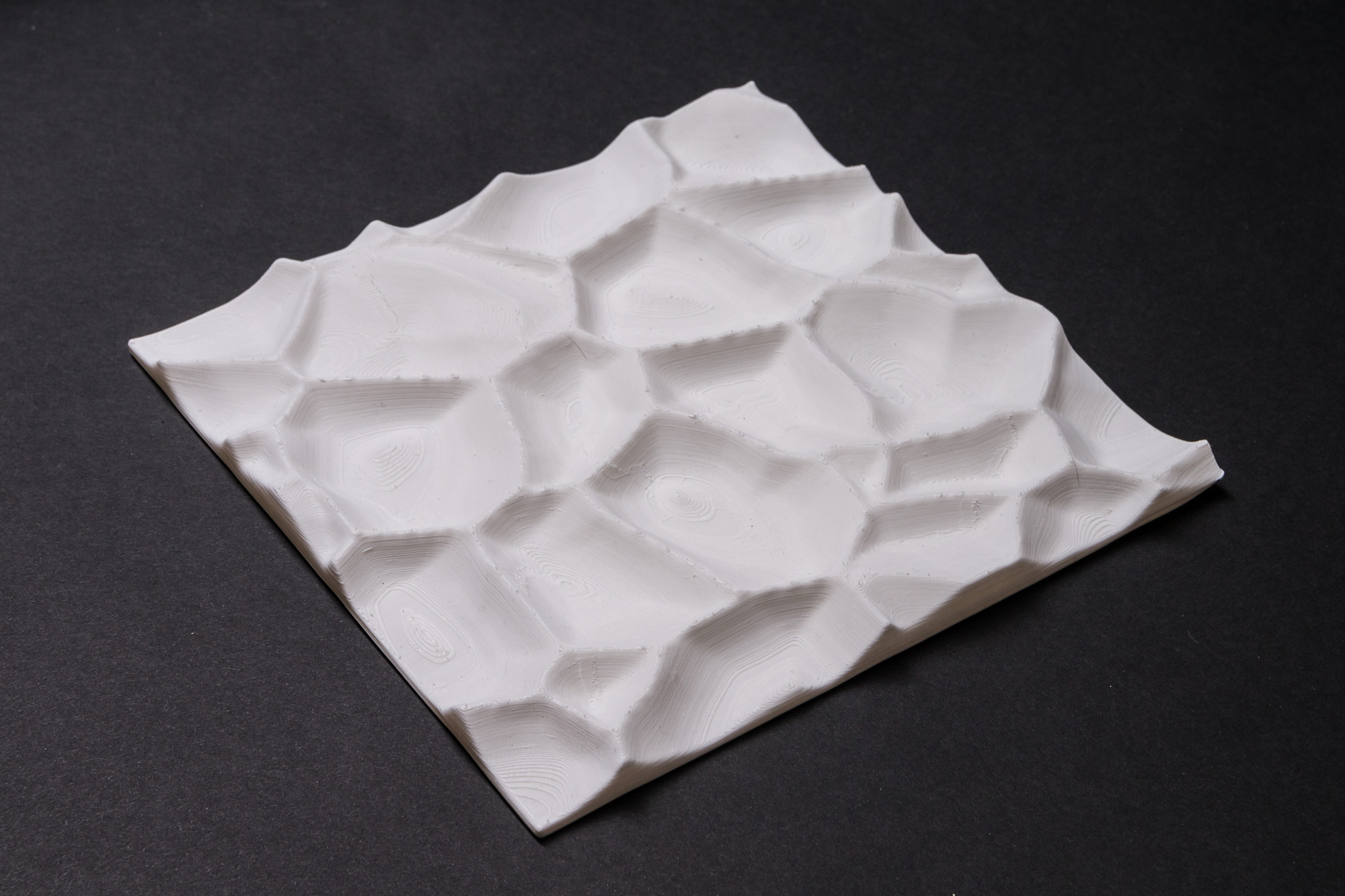
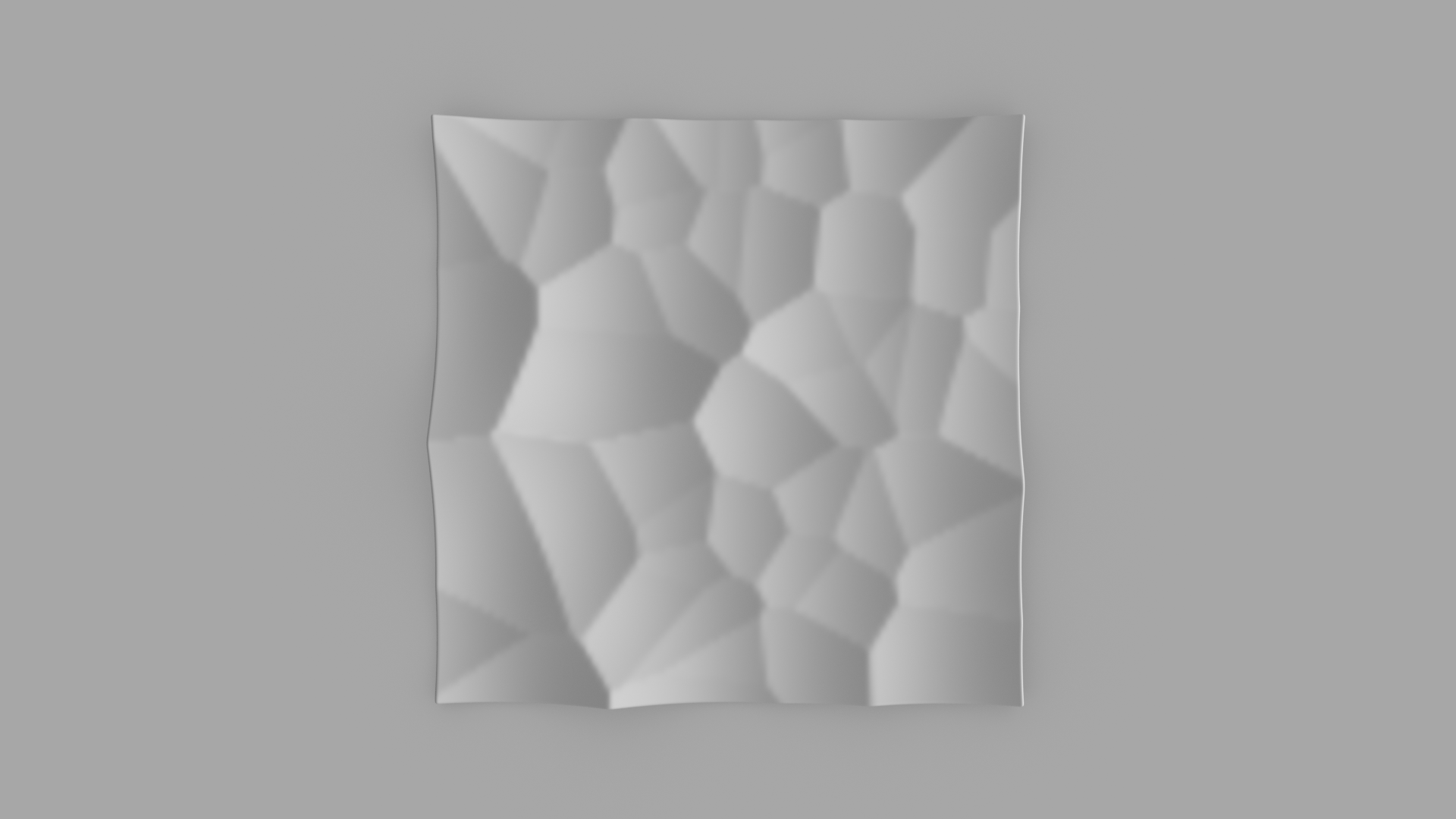
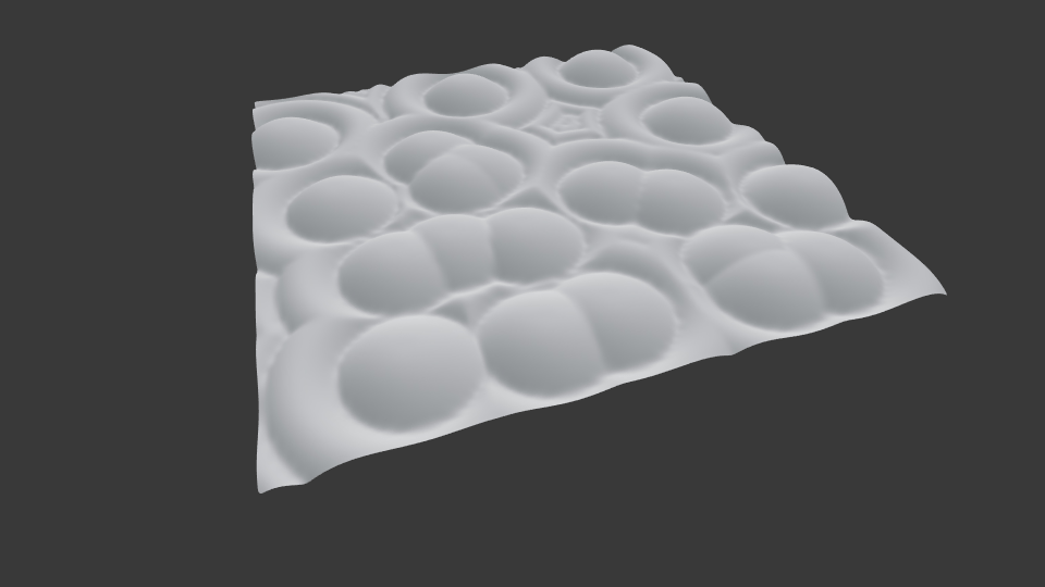
If, instead of working with a 2D image we use a heavily subdivided plane in the 3D space and instead of changing the pixel color we change the Z value of the plane’s vertices, we can get interesting shapes, like this one:
In this tutorial we will see how to obtain the above results with Blender and Sverchok. I have to admit that I spent few hours to get the node tree that implements the algorithm from scratch right, only to find out five minutes later that I could get the same result with few nodes thanks to Variable Lacunarity. I am going to describe both methods anyway, just in case. If you are interested only in getting the result quickly, you can skip the following part.
Raster Voronoi: the long way
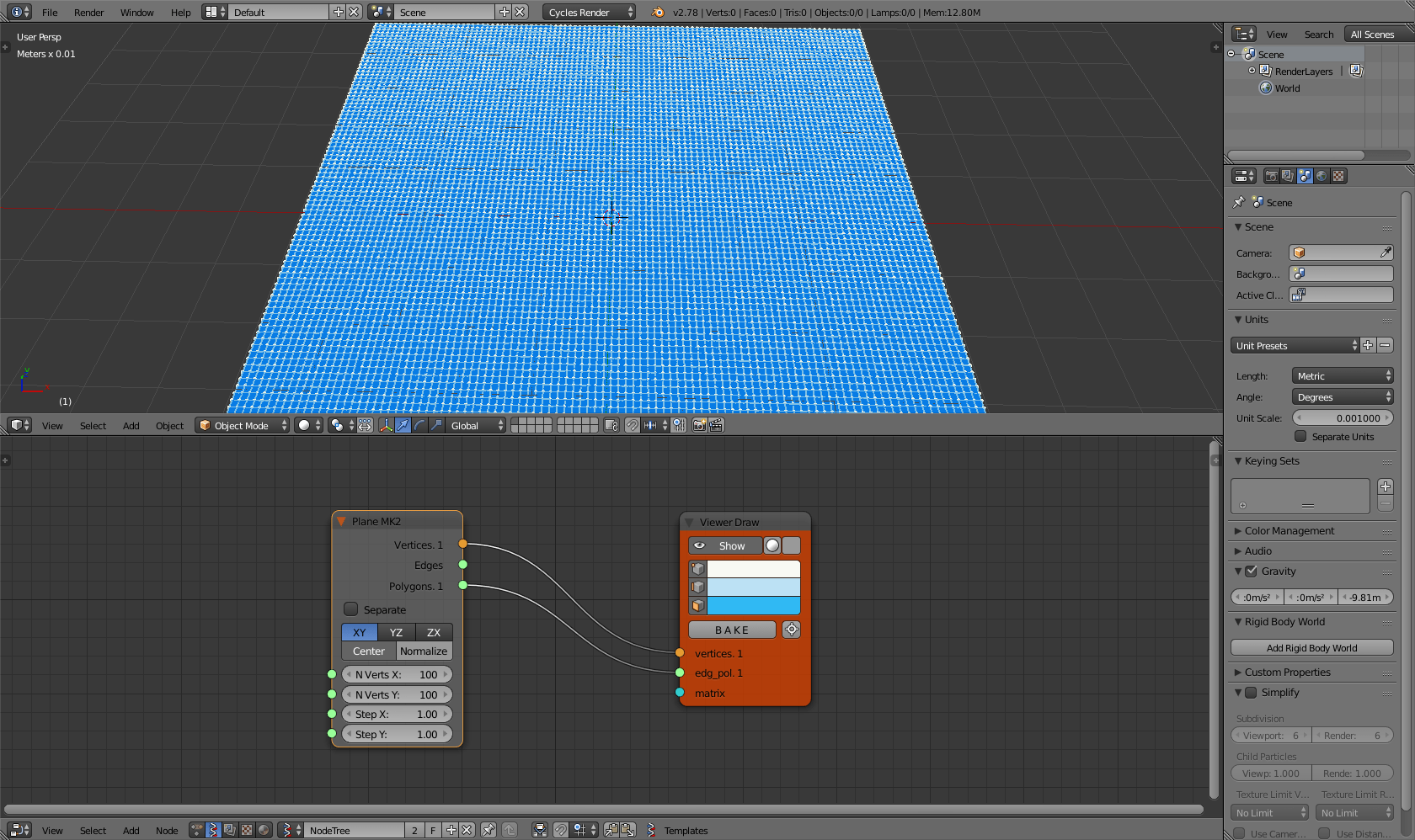
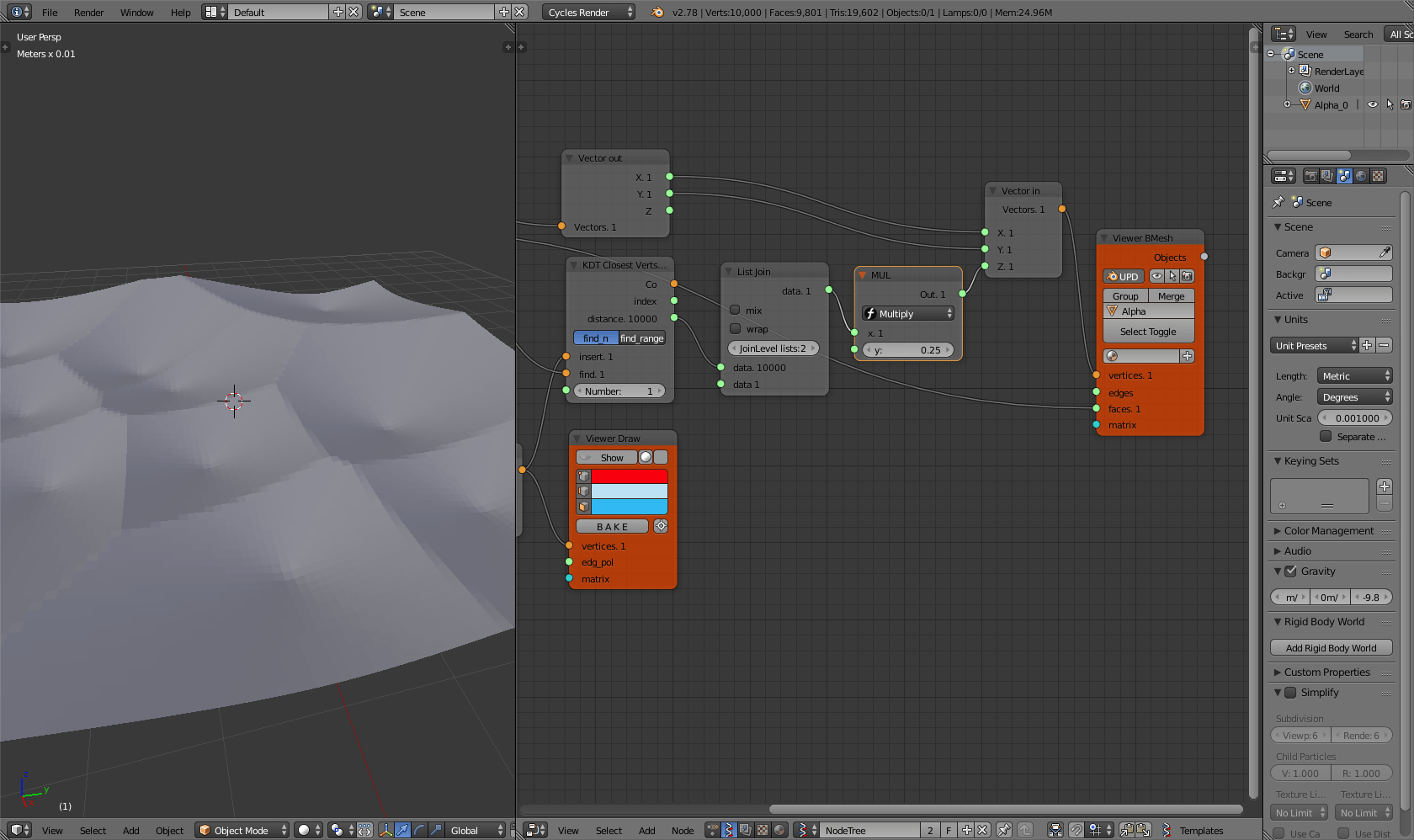
Let’s start from a plane. 100 vertices per sides will be enough.
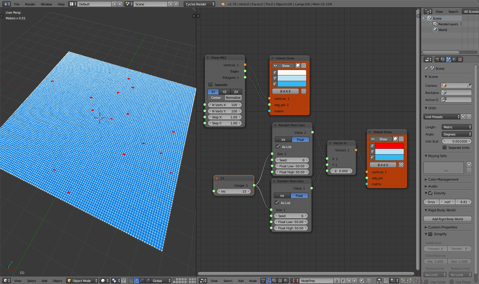
Now we need to add some random points, on which the diagram will be built.
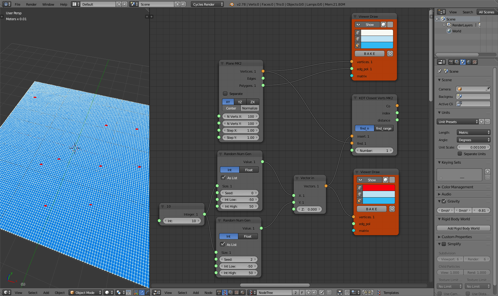
Now we want get the distances to the closest point for each fraction of the plane. Luckily we have a node that allows that: KTD Closest Verts MK2 under the Analyzer group. Plug it in this way:
Within the results you will get the list of the distance from the closest points. Before using this numbers as Z values for the plane’s vertices, it is important that you pass the result through a List Join. Apply a Viewer text node before and after the join to understand the difference. If you don’t do this step, you will crash Blender. Now, using Vector out / Vector in, apply the value to the Z axes of the plane’s vertices.
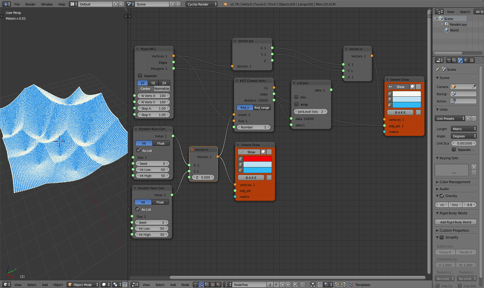
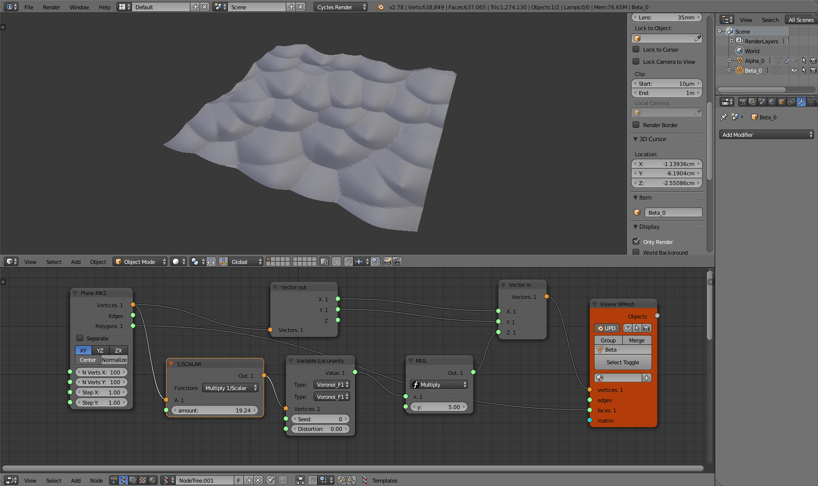
That’s it. Now we can adjust the result in order to make it look nicer. The simplest thing is to multiply the distances value for a reduction parameter (here I have also change the Viewer Draw to a Viewer BMesh).
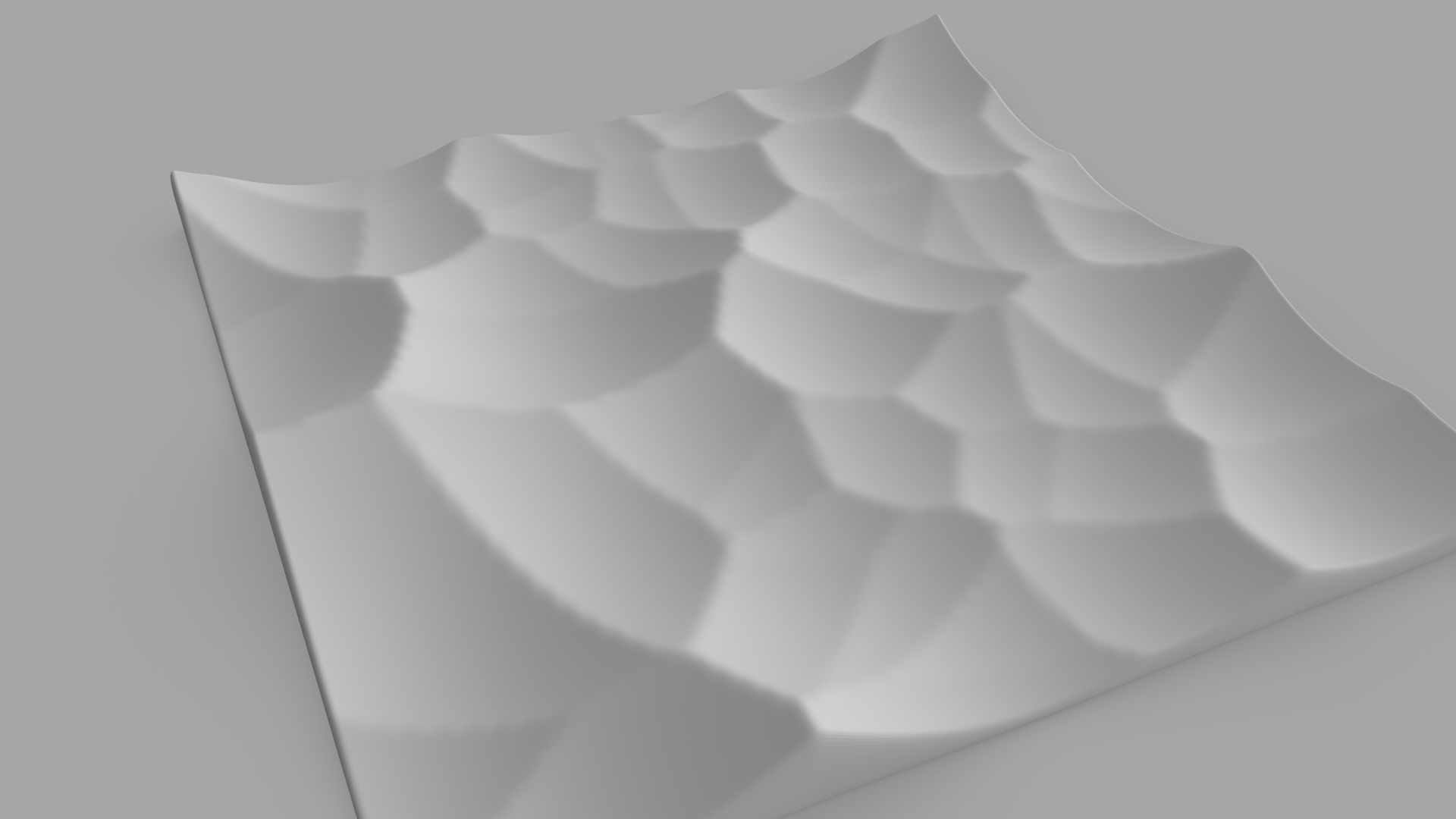
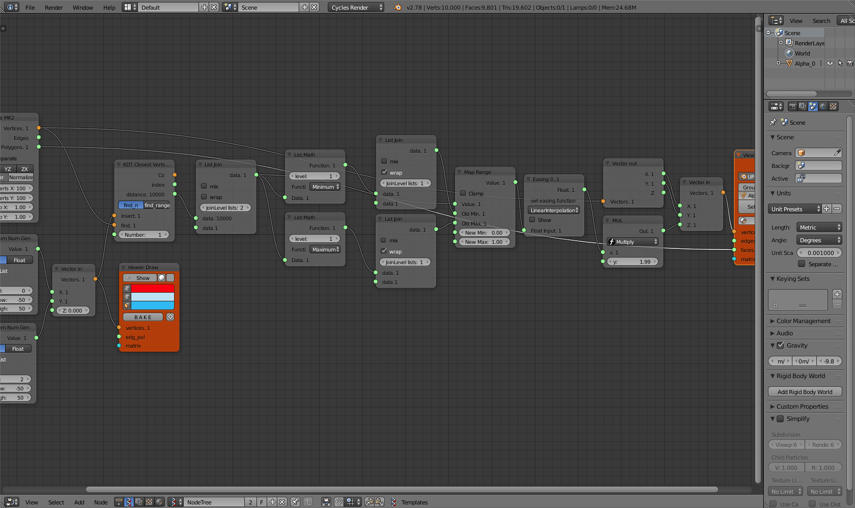
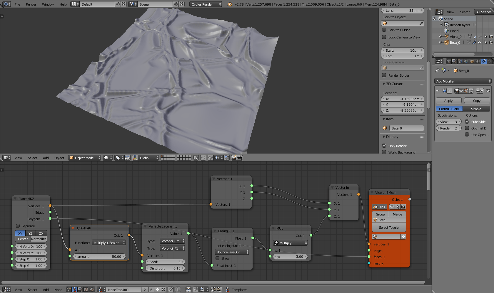
Or, with few extra nodes, we could remap the values so that we can pass them to an Easing 0..1 node to get even more variation on the results. Finally, add a Subdivision surface modifier to the object created by Viewer BMesh to improve the look of it.
Raster Voronoi: the short way
The short way goes like this: we start here too from a subdivided plane.
Plug the Vector out and Vector in nodes to the plane’s vertices and feed the Z value of the Vector in with the output of a Variable Lacunarity node that is fed as well from the plane’s vertices. Variable Lacunarity provides values between 0 and 1, so to make the effects visible, multiply them by some factor.
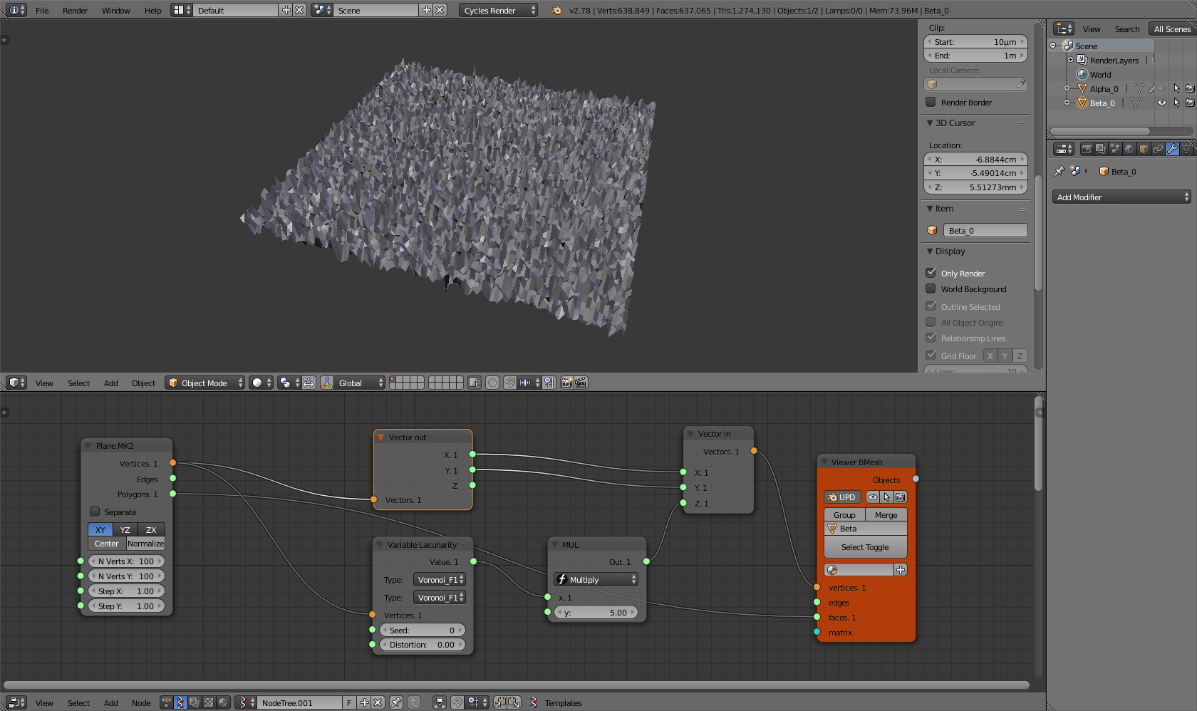
As you can see the results are not very exciting yet. That’s because Variable Lacunarity needs to receive small values in order to output values that are not pure noise. We can achieve this result by multiplying the input vectors by some small scalar. In order to be able to fine tune the end result, I recommend to use the Vector math node with the Multiply 1/Scalar function.
It’s him, our raster Voronoi! The Variable Lacunarity node actually allows much more variation than the method that I have described earlier because we can add a Distortion to our result as well as using different kind of interesting noises, also with the possibility of mixing them together. And to get even more different and spectacular results, let’s pass the output of Variable Lacunarity though a Easing 0..1 node. Remember to add a Subdivision surface modifier to get a smooth mesh.
Now that we have done all this stuff, it is time to use it! How about converting this surfaces in decorative tiles to 3d print or CNC mill? Have fun!